Neural Network Notes: Coding CNN
Last time, I summarized my learnings of the basic concepts of Convolutional Neural Networks (CNNs) and a basic neural network implementation from scratch. In this post, I will continue sharing my experience and notes on coding a CNN from “scratch”, which is still part of my nn-learn project.
The Structure of the Code
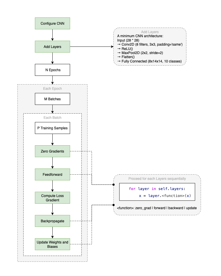
The basic code structure of the CNN is very similar to the basic neural network implementation, but with dedicated network layers and functionalities specific to CNNs. See the diagram below for an overview of the code structure.
The main components include:
- Layer Classes: Each layer type (e.g., convolutional, pooling, fully connected, etc. - details in the section below) is implemented as a separate class, encapsulating its forward and backward pass logic, an optional update function to adjust weights and biases, and a reset gradients function.
- ConvNet Class: The
ConvNetclass manages the overall architecture, including adding layers and providing the SGD training process. - Training Process: The training process is handled in a loop of total N epochs, each epoch runs the whole training dataset, which split into batches, and each batch of data is passed through each layer of the network in the forward pass, gradients for each layer are computed in the backward pass, and at the end of each batch processing the weights and biases are updated based on the computed gradients.
The Key Layers of the CNN Implementation
Convolutional Neural Networks are commonly made up of only three layer types: CONV, POOL (assuming max pooling), and FC (fully connected). However, in practice, CNNs often explicitly write ReLU activation function as a separate layer, which applies element-wise non-linearity, and a Flatten layer to convert the multi-dimensional feature maps into a one-dimensional vector before passing it to the fully connected layer.
Then, the key layers of the CNN implementation in this exercise can be summarized as below:
-
Convolutional Layers: These layers apply convolution operations to the input, allowing the network to learn spatial hierarchies of features. Each convolutional layer is defined by its number of filters, and kernel size.
-
Pooling Layers: Pooling layers reduce the spatial dimensions of the feature maps, helping to down-sample the representation and reduce the number of parameters. Max pooling is commonly used, which takes the maximum value in each patch of the feature map.
-
Activation Functions: Non-linear activation functions, such as ReLU (Rectified Linear Unit), are applied after each convolutional layer to introduce non-linearity into the model.
-
Flatten Layers: After the convolutional and pooling layers, the multi-dimensional feature maps are flattened into a one-dimensional vector to be fed into fully connected layers.
-
Fully Connected Layers: After several convolutional and pooling layers, the high-level reasoning in the neural network is done via fully connected layers. These layers connect every neuron in the previous (flattened) layer to every neuron in the final output layer.
-
Softmax and Loss Function: The loss function measures the difference between the predicted output and the true output. One of the loss functions for classification tasks and also used in this implementation is the Cross-Entropy loss. And before applying the loss function, the Softmax function is often applied to the output layer to convert the raw logits into probabilities.
Backpropagation in CNNs
Now, we come to the most important and interesting part of the CNN implementation: the backpropagation algorithm. Essentially, the 4 fundamental backpropagation equations from Michael Nielsen’s book are still applicable, but with some modifications to accommodate the convolutional and pooling layers, and also the explicitly separated ReLU layer. The key idea of backpropagation in CNNs is still the same,
- First, compute the gradients of the loss function with respect to the output (the logits) of the network.
- Then, propagate these gradients backward through the network, layer by layer. Specifically, there are at most 3 different gradients to calculate for each layer:
- The gradient of the loss with respect to the weights of the current layer.
- The gradient of the loss with respect to the biases of the current layer.
- The gradient of the loss with respect to the input of the current layer, which will be used as the input for the previous layer in the backward pass. This is the gradient that makes the backpropagation happen through the network.
- For each layer, the gradients are computed based on the specific operations performed in that layer.
- For convolutional layer, the gradients w.r.t. weights are computed by summing the convolution of the input feature maps of current layer with the gradient of input feature maps from the next layer; the gradients w.r.t. biases are computed by summing the gradients of the input feature maps from the next layer; and the gradients w.r.t. input are computed by summing the convolution of the gradient of input feature maps from the next layer with the weights of the current layer.
- For ReLU activation layer, the gradients are computed by applying the ReLU derivative (which is 1 for positive inputs and 0 for negative inputs) to the gradient of the input feature maps from the next layer.
- For Flatten layer, the gradients are simply reshaped to match the shape of the input feature maps.
- For fully connected layers, the gradients w.r.t. weights are computed by multiplying the input feature maps of current layer with the gradient of input feature maps from the next layer; the gradients w.r.t. biases are equal to the gradients of the input feature maps from the next layer; and the gradients w.r.t. input are computed by multiplying the gradient of input feature maps from the next layer with the transpose of the weights of the current layer.
- For pooling layer, the gradients are propagated back to the input based on the indices of the maximum values in the pooling operation.
- Finally, the gradients of the weights and biases are used to update the parameters of the network.
📝 Notes
The gradients of the weights and biases need to reset to zero before each batch processing, otherwise the gradients will accumulate across batches, which is not what we want. This is done in the
zero_gradfunction for layers having trainable parameters (e.g., convolutional and fully connected layers).
Training and Optimizations
Then, we can start to construct our CNN model by adding layers flexibly, but following this common layer patterns: INPUT -> [[CONV -> RELU]*N -> POOL?]*M -> [FC -> RELU?]*K -> FC. I started with a simple CNN model with minimum layers: INPUT -> CONV -> RELU -> POOL -> (Flatten) -> FC, which is already surprisingly effective to achieve a decent accuracy - higher than 97% on the MNIST dataset.
However, I also noticed the training process was quite slow even with the minimum layers architecture and training on the small MNIST dataset. Compared to the previous basic neural network implementation, the speed of training was significantly slower about 3 orders of magnitude. This is mainly due to the fact that the convolution operation is computationally more expensive than the matrix multiplication in fully connected layers, and the backpropagation through convolutional layers is also more complex.
To speed up the training process, I mainly applied these 2 optimizations:
- Batch Processing: Instead of processing one sample at a time, I implemented batch processing, which allows the network to process multiple samples in parallel. However, this does not significantly speed up the training process, as the convolution operations are still processed in simple loops.
- Vectorization: Then, I learned that vectorized convolution is an optimization technique where the standard nested-loop-based convolution operation can be rewritten using numpy’s vectorized operations, which are much faster than using simple loops. This is a crucial optimization, as Numpy’s vectorized operations are implemented in C and can take advantage of low-level optimizations, making them much faster than Python loops.
After applying these optimizations, the training speed increased about 100 times, allowing me to try more complex CNN architectures and achieve even higher accuracy on the MNIST dataset. I will share my test results right in the next section.
📝 Notes
The vectorized convolution implementation is much complex than I thought, which though I’ve implemented them in the code with the help of Copilot, I haven’t fully understood the details yet. Mainly because I am still new to Numpy’s n-dimensional arrays and their advanced operations. This deserves another dedicated learning session in the future. But for now, let me just leave it here.
Test Results
The test results for the 2 CNN models are summarized in the table below. The first model is a simple CNN with minimum layers, and the second model is a more complex CNN with additional convolutional and fully connected layers. Both use the same training dataset MNIST and hyperparameters (batch_size=10, learning_rate=0.05, epochs=30), and the training process is done on CPU.
| Model | Architectures | Accuracy | Training Time |
|---|---|---|---|
| Simple CNN | Input (28x28) |
97.67% | ~ minutes |
| Complex CNN | Input (28x28) |
99.33% | ~ hours |
📝 Notes
The test script can refer to here, and run
python3 test.py convnetfor the simple CNN model, andpython3 test.py convnet complexfor the complex CNN model.
A Brief Notes about Numpy N-D Arrays
Numpy’s n-dimensional arrays (ndarrays) are a powerful feature that allows for efficient storage and manipulation of large datasets. Here are some key points to remember when working with ndarrays, especially in the context of CNNs:
- Shape and Dimensions: Numpy arrays can have any number of dimensions, and the shape of an array is defined by a tuple of integers representing the size of each dimension. For example, a 2D array (matrix) has a shape of
(rows, columns), while a 3D array (like an image with RGB channels) has a shape of(channels, height, width). - Axes: Each dimension of a Numpy array is referred to as an axis. The first axis (axis 0) starts at the outermost dimension, and subsequent axes increase in depth. For example, in a 3D array representing an image, axis 0 can represent the color channels (e.g., RGB), axis 1 the height, and axis 2 the width.
- Indexing and Slicing: Numpy arrays support advanced indexing and slicing, allowing you to access and modify specific elements or sub-arrays efficiently. For example,
array[0, 1]accesses the element at row 0 and column 1, whilearray[:, 1]accesses all elements in column 1 across all rows. - Broadcasting: Numpy’s broadcasting feature allows you to perform operations on arrays of different shapes without explicitly reshaping them. This is particularly useful in CNNs when you want to apply operations across different dimensions, such as adding a bias term to a weighted sum of receptive fields of the inputs.
- Reshaping: You can reshape an array using the
reshapemethod, which allows you to change the shape of an array without changing its data. This is useful when flattening feature maps before passing them to fully connected layers in CNNs. - Memory Layout: Numpy arrays can be stored in either row-major (C-style) or column-major (Fortran-style) order. Understanding the memory layout can help optimize performance, especially when dealing with large datasets or complex operations.
What is Next?
Although I have implemented a basic CNN from “scratch” and achieved a decent accuracy on the MNIST dataset, there are still many areas to explore further, such as applying dropout layer to prevent overfitting, employing batch normalization layer to stabilize training, introducing momentum or Adam optimizer to speed up convergence, and use more advanced datasets. But, right now I think I am quite satisfied with the current learnings and explorations on CNNs, so I will switch the gear to other topics, such as ResNet, Recurrent Neural Networks (RNN), and Transformers.
Blogging will continue after I have enough learnt about these new topics, but I will just conclude this blog for now.