How I Learn Diffusion Model
It has been over three months since my last post on building a toy Transformer from scratch. At the time, I was torn between two paths: diving deeper into more theoretical knowledge of AI or getting hands-on with real-world projects using agentic AI. Ultimately, I was pulled in the direction of exploring another intriguing subject: Diffusion Models.
To be honest, it is a daunting topic. It demands a level of mathematical depth that I haven’t yet mastered, but to understand the mathematics behind it is just what drives me. I am still in the early stages of this journey, but I want to document and share the things I have learned so far.
Where I Started
The first time I experienced the “magic” of text to image generation was through the DALL-E model from OpenAI and in the Discord group of Midjourney almost 4 years ago. Though it was very impressive, it didn’t trigger my immediate interest, until the Stable Diffusion was released by Stability AI, which also open-sourced the code and model weights. And its the mechanism of creating high-quality images from pure Gaussian noise really caught my deep curiosity.
This was where I started, and finally I decided to spend most of my spare time in the past 3 months learning the diffusion model.
The Learning Plan
After several days of exploring the web, reading blog posts, and consulting with LLMs, I have converged on a learning path structured into five key stages:
- Conceptual Foundations: This guest youtube video from 3Blue1Brown gives a good general introduction to diffusion models, besides there are also a ton of good resources listed in the video description. Furthermore, this MIT open course Generative AI - Text-to-Image Models provides a slight more technical yet still accessible introduction to this topic, but still at an entry level.
- Mathematical Explanation: This is where the real challenge lies. I initially dove into lilianweng’s blog post What are Diffusion Models? and the original paper Denoising Diffusion Probabilistic Models by Ho et al. However, I quickly realized I am not equipped with the necessary mathematical knowledge to understand the flow of the explanation or the descriptions in the paper. This led me to this comprehensive online course MIT 6.S184: Flow Matching and Diffusion Models by Peter Holderrieth - a systematic and rigorous resource for understanding the mathematical foundations of flow matching and diffusion models.
- Model Architecture: The next goal is to understand the model architecture, specifically the U-Nets and Diffusion Transformers (DiTs), about how they are structured and trained.
- Guided Generation: After understanding the basic architecture, I want to explore how to guide the generation process with additional conditions, such as text prompts. This is a crucial aspect of diffusion models that allows for more control and creativity in the generated outputs.
- Hands-on Implementation: As usual, after understanding the theoretical aspects well enough, I will try to implement a toy diffusion model from scratch.
- Evolution and Research: Finally, I want to trace the development history of this field to fulfill my curiosity of the process of discovery, and keep up with the latest research papers and advancements in diffusion models, to understand how the field is evolving and where it might be headed in the future.
At this point, I am deep in the second stage. Navigating the mathematical theory behind the model is a big challenge for me, as I had to pause frequently to build the knowledge base of relevant maths in Probability Theory, Ordinary and Stochastic Differential Equations, Multivariate Normal Distribution, Variational Bayesian methods, etc. The goal is not to become a math expert in these areas, but to reach a level where I can understand the mathematical explanations in the original papers and many of the great blog posts out there without much difficulty. I think I am making some progress, but it is still a long way to go.
What I Understand So Far
The learning notes I took here focus on the specific construction of generative models using flow models, which is trained using flow matching loss.
The Mathematical Definition of the Problem
Given a set of samples $x_1, x_2, \ldots, x_n$ drawn from an unknown, high dimensional data distribution $p_{data}$, how do we build a generative model that can generate new samples that looks like they are drawn from the same data distribution?
Introduce Flow Models
The generative model can be constructed by flow models. A flow model is described by the Ordinary Differential Equation (ODE):
\[X_0 \sim p_{init} \tag{random initialization}\] \[\frac{dX_t}{dt} = u_t(X_t) \tag{ODE}\]where the ODE is defined by a vector field $u_t$. The goal is to make the endpoint $X_1$ of the flow have distribution $p_{data}$. And the learning target is the vector field $u_t$, which is parameterized by the neural network as $u^{\theta}_t$.
Once we have the learned vector field $u^{\theta}_t$, we can then generate new samples by simulating the ODE with Euler method:
\[X_{t+h} = X_t + hu^{\theta}_t(X_t)\]Where $h$ is the step size. By iterating this process from $t=0$ to $t=1$, we can obtain a sample $X_1$ that is approximately drawn from the data distribution $p_{data}$.
Define Probability Paths
To connect the vector field with the data distribution, we need to define a probability path $p_t(x)$ that evolves over time from the initial distribution $p_{init}$ to the data distribution $p_{data}$. Intuitively, a probability path specifies a gradual interpolation between the initial distribution and the data distribution. One particularly popular choice is the Gaussian propability path. The conditional Gaussian probability path is defined as:
\[p_t(\cdot | z) = \mathcal{N}(\alpha_t z, \beta_t^2 \mathbf{I}_d)\]Where $\alpha_t$ and $\beta_t$ are time-dependent noise schedules that control the mean and variance of the distribution at time $t$.
The question now is how can we find a vector field $u_t$ that the flow $X_t$ follow the probability path? Usually, the conditional vector field can be analytically constructed from the conditional probability path. For example, for the Gaussian probability path shown above, the corresponding conditional vector field can be constructed as:
\[u_t(x|z) = (\alpha_t' - (\beta_t'/\beta_t) \alpha_t)z + (\beta_t' / \beta_t)x\]Where $\alpha_t’$ and $\beta_t’$ are the derivatives of $\alpha_t$ and $\beta_t$ with respect to time $t$.
Marginalization Trick and Continuity Equation
The conditional vector field constructed as above does not help by itself, because all the trajectories of the flow will collapse to the same point $z$, we just regenerate the known data point $z$. However, the conditional vector field serves as a building block for constructing the marginal vector field that can generates actual samples from $p_{data}$. This marginal vector field is defined using the marginalization trick:
\[u_t(x) = \int u_t(x|z) \frac{p_t(x|z) p_{data}(z)}{p_t(x)} dz\]Which follows the marginal probability path,
\[X_0 \sim p_{init}, \quad \frac{dX_t}{dt} = u_t(X_t) \implies X_1 \sim p_{data}\]This connection can be proved by the continuity equation, which states that the change in probability density over time is equal to the negative divergence of the probability flux:
\[\frac{\partial p_t(x)}{\partial t} = - \operatorname{div}(p_t u_t)(x)\]Where the divergence operator is defined as:
\[\operatorname{div}(v_t)(x) = \sum_{i=1}^d \frac{\partial v^i_t(x)}{\partial x_i}\]Learning the Vector Field by Flow Matching Loss
Recall that the learning target is the vector field $u^{\theta}_t$, and the loss function is to use a mean-squared error, defined as the flow matching loss:
\[\begin{align} \mathcal{L}_{FM}(\theta) &= \mathbb{E}_{t \sim \mathcal{U}(0,1), x \sim p_t} \left[ \| u^{\theta}_t(x) - u_t(x) \|^2 \right] \\ &= \mathbb{E}_{t \sim \mathcal{U}(0,1), z \sim p_{data}, x \sim p_t(\cdot|z)} \left[ \| u^{\theta}_t(x) - u_t(x) \|^2 \right] \end{align}\]The calculation will be something like this:
- draw a random time $t$ from a uniform distribution,
- sample a data point $z$ from the data distribution,
- sample a point $x$ from the conditional probability path \(p_t(\cdot|z)\),
- compute the vector field $u^{\theta}_t(x)$ by the neural network,
- finally, compute the loss between $u^{\theta}_t(x)$ and $u_t(x)$.
Seems straightforward, but the target vector field $u_t(x)$ is intractable. However, we can use the conditional vector field \(u_t(x|z)\) to construct an unbiased estimator of the loss:
\[\begin{align} \mathcal{L}_{CFM}(\theta) &= \mathbb{E}_{t \sim \mathcal{U}(0,1), z \sim p_{data}, x \sim p_t(\cdot|z)} \left[ \| u^{\theta}_t(x) - u_t(x|z) \|^2 \right] \end{align}\]This is valid because the marginal flow matching loss equals the conditional flow matching loss up to a constant:
\[\mathcal{L}_{FM}(\theta) = \mathcal{L}_{CFM}(\theta) + C\]Therefore, flow matching training consists of minimizing the conditional flow matching loss.
Flow Matching for Gaussian Probability Paths
At last, let us take a look at the specific case of Gaussian probability paths for calculating the flow matching loss.
- Choose the Gaussian probability path \(p_t(\cdot | z) = \mathcal{N}(\alpha_t z, \beta_t^2 \mathbf{I}_d)\).
- Sample $x_t$ from $X_t \sim \alpha_t z + \beta_t \epsilon$, where $\epsilon \sim \mathcal{N}(0, \mathbf{I}_d)$.
- The conditional vector field of $X_t$ can be derived as: \(u_t(x|z) = (\alpha_t' - (\beta_t'/\beta_t) \alpha_t)z + (\beta_t' / \beta_t)x\).
-
Then, plug the above formulas into the conditional flow matching loss:
\[\begin{align} \mathcal{L}_{CFM}(\theta) &= \mathbb{E}_{t \sim \mathcal{U}(0,1), z \sim p_{data}, x \sim p_t(\cdot|z)} \left[ \| u^{\theta}_t(x) - (\alpha_t' - (\beta_t'/\beta_t) \alpha_t)z - (\beta_t' / \beta_t)x) \|^2 \right] \\ &= \mathbb{E}_{t \sim \mathcal{U}(0,1), z \sim p_{data}, x \sim p_t(\cdot|z)} \left[ \| u^{\theta}_t(\alpha_t z + \beta_t \epsilon) - (\alpha_t' z + \beta_t' \epsilon) \|^2 \right] \\ \end{align}\] -
Finally, let’s make the noise schedule concrete by choosing $\alpha_t = t$ and $\beta_t = 1 - t$, then we have $\alpha_t’ = 1$ and $\beta_t’ = -1$, so that the loss can be simplified as:
\[\begin{align} \mathcal{L}_{CFM}(\theta) &= \mathbb{E}_{t \sim \mathcal{U}(0,1), z \sim p_{data}, x \sim p_t(\cdot|z)} \left[ \| u^{\theta}_t(t z + (1-t) \epsilon) - (z - \epsilon) \|^2 \right] \\ \end{align}\]
A Quick Visual Summary
The hand-written diagram below demonstrates how I put them altogether:
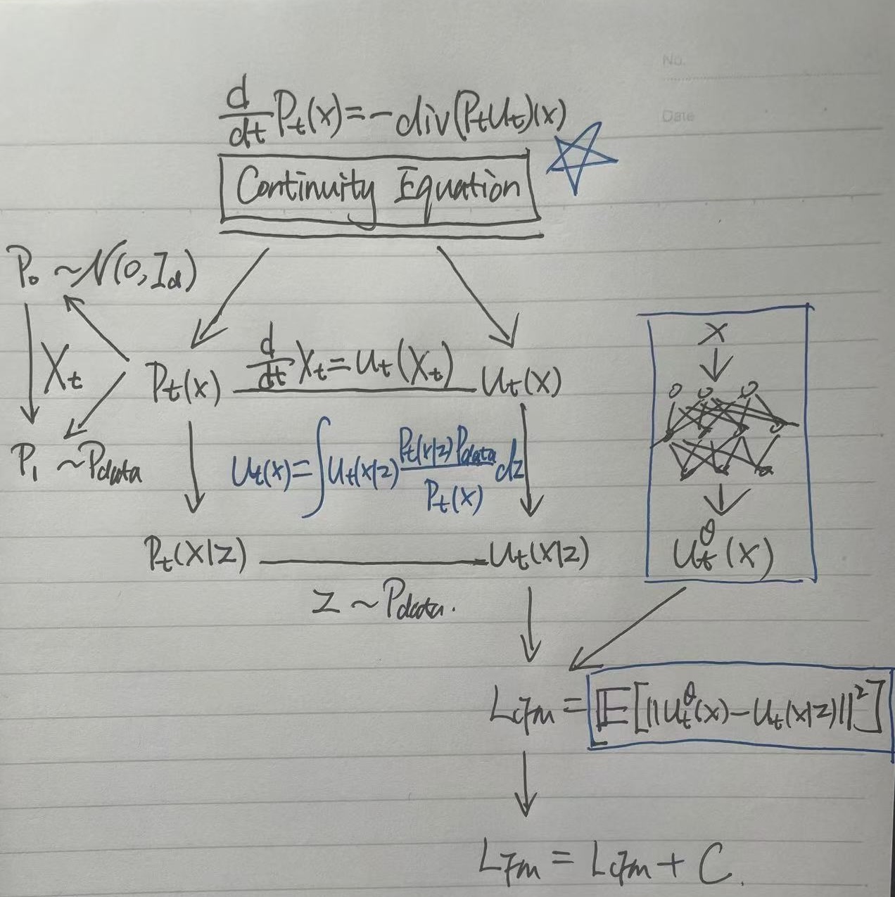
- The Continuity Equation as the Foundation: It serves as the fundamental principle (the “glue”) that ensures the evolution of the probability density $P_t$ is consistent with the underlying velocity field $u_t$.
- Defining the Probability Path: We construct a conditional probability path (typically Gaussian) that bridges the source (Gaussian noise $P_0$) and the target (data distribution $P_1$). While the marginal path $P_t(x)$ is complex and intractable, the conditional path $P_t(x|z)$ is simple and easy to sample.
- Vector Field Correspondence: For the probability path, there exists a corresponding vector field $u_t$ that generates that flow evolving along the path. And this vector field is the learning target for the neural network.
- Tractability via Conditional Flow Matching (CFM): Since the true marginal vector field $u_t(x)$ is impossible to compute directly, we use the Conditional Flow Matching loss. This allows us to regress against the conditional vector field $u_t(x|z)$, which can be derived analytically from our chosen Gaussian probability path.
- Loss Equivalence: Minimizing the CFM loss is mathematically equivalent to minimizing the true Flow Matching (CF) loss (up to a constant). Thus, by training on the conditional target, the neural network learns a marginal vector field that correctly transitions noise to the data distribution along the intended path.
The Big Question
Though I have generally understood the mathematical construction of the flow model, the big question still remains: Why does this whole thing actually work?
- Why the mathematical definition of this generative model is defined as learning the unknown data distribution and sampling from it?
- How was the ODE method introduced in the first place, and further discovered the vector field to be the learning target?
- Why the popular Gaussian probability path is chosen, and can work surprisingly well?
All in all, it is still astonishing to me that we can generate high-quality images from pure Gaussian noise by learning the vector field that follows a simple Gaussian probability path.
Conclusion and Next Step
I feel like I’ve only just scratched the surface of this generative model. While my current focus is on Flow Matching, there are also many other mathematical frameworks designed to reach the same goal — learning a data distribution from noise. I’ve come across the Markov Chain perspective from the original DDPM paper, DDIMs and their use of ODEs, and the Score Matching approach using SDEs. That’s not even mentioning the predecessors like VAEs and GANs, which each carry their own unique mathematical constructions.
I’ll be leaving those topics for a later time to keep my focus on Flow Matching, which represents the current state-of-the-art. And my next step will follow the learning plan I outlined above, and a separate blog post may be written when I feel I have enough new learnings to share.