Neural Network Notes: Coding the Network from Scratch
I’ve set out on a journey to learn and understand AI — with the ultimate goal of grasping the essence of large language models (LLMs) and exploring the frontier of research in this field freely. This pursuit is driven by a deeper curiosity: a desire to understand the origins of human consciousness. I believe that advances in AI and the ongoing quest to develop artificial general intelligence (AGI) can offer valuable insights into this profound question.
To begin this journey, I started by studying the fundamentals of neural networks and the backpropagation algorithm, followed by an introduction to convolutional neural networks.
Before moving further, I want to solidify my understanding by getting hands-on — coding a basic neural network with the backpropagation algorithm from scratch. I’ll be using and learning from the excellent code example in the online book Neural Networks and Deep Learning. My goal is to truly grasp the core mechanism that powers a neural network’s ability to learn.
Then, I’ve started this github repo - nn-learn for managing my code implementation of the learning. And this blog is to document the experience of coding a basic neural network along the way.
The Structure of the Code
Surprisingly, fewer than 100 lines of Python code are enough to build a basic neural network architecture, implement the training loop, and update weights and biases effectively using stochastic gradient descent (SGD) combined with the backpropagation algorithm. Thankfully, Python’s NumPy library makes matrix operations significantly easier and more efficient.
After just a few dozens training iterations, the network is already able to predict handwritten digit images with impressive accuracy — often exceeding 95%.
The diagram below provides a visual overview of how the training code is structured:
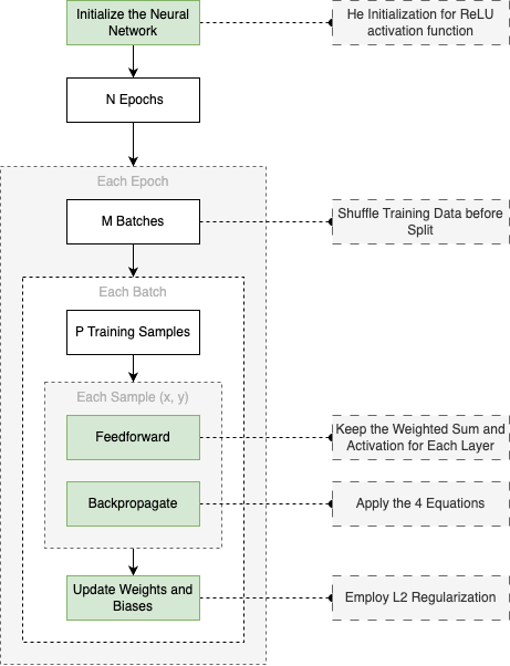
To be clear, I didn’t write all of this entirely from scratch. I referred to the code example from the excellent online book Neural Networks and Deep Learning by Michael Nielsen (mentioned earlier). My modified version of the implementation can be found in this file in my GitHub repo, where I’ve added extra comments, rearranged the code a bit, following my own learning process.
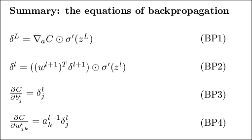
One part I want to highlight here is the backpropagation function. I’ve annotated each step of the code with references to the corresponding equations from the book:
📝 Notes
I modified the original code to allow using different activation functions for the hidden and output layers, enabling experiments to observe how various activations affect training results.
    def _backprop(self, y):
        """
        Backpropagation algorithm to compute gradients.
        :param y: Target output
        """

        """
        Calculate the gradient of the cost function with respect to
        the output of the network.
        Apply equation (BP1)
        """
        delta = self.cost_fn.prime(y, self.activations[-1]) * \
                self.activation_fns['output'].prime(self.zs[-1])
        """
        Apply equation (BP3) and (BP4)
        """
        self.nabla_b[-1] += delta
        self.nabla_w[-1] += np.dot(delta, self.activations[-2].T)

        """
        Iterate through the layers in reverse order to compute gradients
        """
        for l in range(2, self.size):
            z = self.zs[-l]
            sp = self.activation_fns['hidden'].prime(z)

            """
            Apply equation (BP2)
            """
            delta = np.dot(self.weights[-l + 1].T, delta) * sp

            """
            Apply equation (BP3) and (BP4)
            """
            self.nabla_b[-l] += delta
            self.nabla_w[-l] += np.dot(delta, self.activations[-l - 1].T)
The four fundamental equations used above are explained in detail in the book and were also discussed in my earlier blog post, where I gave the complete proof.
Exploring Activation Functions and L2 Regularization
The initial version of the neural network was quite straightforward: it used the sigmoid activation function for all layers, a quadratic cost function for computing loss, and initialized weights and biases with a standard normal distribution. Even with this simple setup, training a network with 30 hidden neurons for 30 epochs already yielded solid results — around 95% accuracy on the validation set.
To explore whether I could push the performance further, I experimented with changing the activation function. After reading that ReLU is often preferred in deeper networks due to its ability to mitigate the vanishing gradient problem common with sigmoid, I replaced the hidden layer activation function with ReLU while keeping the output layer unchanged.
At the same time, I introduced L2 regularization into the cost function to help reduce overfitting and improve the model’s ability to generalize. Since switching to ReLU can lead to the “dying ReLU” problem — where some neurons stop activating and effectively become untrainable — I adjusted the weight initialization using He initialization to mitigate this risk. Interestingly, this issue was one of the challenges I ran into during experimentation, which I describe in more detail in the next section.
After these updates were properly configured, the network’s accuracy improved to around 96.33%. That may not seem like a huge jump at first glance, but in this context, gaining over 1% in accuracy was a clear indication that these adjustments made a real impact.
Challenges Along the Way
The biggest challenge I faced was not knowing where to start debugging when things didn’t work as expected. This happened immediately after I hit “Enter” to start the training process with my first implementation. The accuracy on the validation data set remained stuck at 10% after each epoch — a clear sign that the neural network wasn’t learning at all. The weights and biases still appeared to be random, suggesting that the training had no effect.
Such situation is particularly difficult for a beginner, because I could be wrong in many naive ways. The facts have also proved this. Here’s a list of what I got wrong,
- I unintentionally reversed the order of matrix multiplication in Equation 2, which fortunately triggered a runtime error that helped me catch it early.
- I mistakenly used the cost function itself where I should have used its derivative in Equation 1.
- There was a bug in my evaluation code — I misused NumPy’s argmax function, which led to incorrect outputs even though the network was actually trained correctly.
- I also ran into some minor issues simply due to my unfamiliarity with certain NumPy data structures and operations.
To catch these low-level bugs, I relied on two basic but effective strategies: carefully re-reading the code and printing out anything that looked suspicious for verification. After a few rounds of this (read → print → verify) cycle, the bugs were gradually ironed out.
Once the basic neural network started working, I moved on to experimenting with different configurations. But new problems surfaced. One significant issue arose after I literally switched to the ReLU activation from the Sigmoid function. The training accuracy dropped drastically — sometimes even below 50%. At first, I felt stuck. With so many weights, biases, and activations involved, printing them for each mini-batch update resulted in pages of output. It felt impossible to analyze or reason about those values by eye — at least not for me, at this stage.
Still, I had no better option, so I started printing out weights and activations for certain iterations. It turned out that many neurons in the hidden layer had activations stuck at zero after just a few training iterations. This was a red flag.
After some research, I learned about the “dying ReLU” problem — a common issue where ReLU neurons become inactive due to consistently negative weighted inputs, resulting in both zero gradients and zero activations (no learning). To mitigate this, I adopted He initialization for the weights and also reduced the learning rate, which helped bring the network back on track again.
Excitement to See - It Works!
Now comes the moment of joy — the moment when everything finally comes together, and the neural network not only trains successfully but also predicts new inputs with remarkable accuracy. That sense of accomplishment reminded me of the simple joy I felt when building things as a kid — except now, it was backed by actual math and code.
What made it especially rewarding was seeing how concepts I had read about — like forward propagation, backpropagation, and SGD — translated into working code. It’s one thing to follow a tutorial or read through equations, but it’s a completely different experience to implement the pieces yourself and watch them work as expected.
At the same time, it was also a good reminder of how much foundational knowledge is packed into even a small project like this. The code may be short, but behind it are decades of research in mathematics, computer science, and neuroscience. I didn’t invent the methods, but by working through them line by line, I gained a deeper appreciation for how everything fits together — and that’s exactly what I was hoping to get out of this learning process.
This is Just the Beginning
This basic neural network is both surprisingly simple in code and surprisingly powerful in performance — achieving impressive accuracy with under a hundred lines of Python. But this is just the beginning.
There’s so much more to explore further: modern deep learning architectures, more sophisticated optimization techniques, transfer learning, and eventually, how large language models are built and trained. The road ahead will no doubt bring new challenges and discoveries, but for now, I’ll take a breath, and conclude this blog here.