Neural Network Notes: Recurrent Neural Network and BPTT
Until now, I am quite happy with the progress of my neural network learning journey. I have covered the basics of neural networks, convolutional neural networks, and also get my hands on coding the vanilla neural network and convolutional neural network from “scratch”. Now, it is time to dive into another innovative architecture: recurrent neural networks (RNNs), a type of artificial neural network designed to process sequential data, where the order of elements is crucial, like text or time series.
📝 Notes
Just a kind reminder to those who occasionally come across my blog: I’m not an expert in neural networks—I’m still learning. This blog and the entire neural network series are mainly a record of my personal learning journey. That said, I’m glad if any part of them is helpful to you as well.
What is a Recurrent Neural Network?
A Recurrent Neural Network (RNN) is a type of neural network specialized for processing sequences, where the order of inputs matters — such as in text, speech, or time-series data. Unlike traditional feedforward networks, RNNs introduce recurrent connections, meaning the output at each time step is fed back into the network to influence future predictions. This feedback loop allows the model to retain a form of memory, making it suitable for tasks involving context and temporal dependencies.
When I first encountered this definition, I found it quite abstract. What exactly does it mean to “feed back” outputs? What does the architecture really look like? These questions, and more, came to mind:
- What does the architecture of a vanilla RNN look like, and how do the recurrent connections work?
- How is backpropagation applied in RNNs, and why are they more prone to the vanishing gradient problem?
- How are RNNs trained for tasks like sequence prediction or text generation?
- How do we use a trained RNN model to generate new text given a seed?
- Can I implement a simple RNN from scratch using just Python and NumPy?
- What are the main RNN variants like LSTM and GRU, and how do they improve over vanilla RNNs?
- How did the development of RNNs lead to attention mechanisms, Transformers, GPT, and modern LLMs?
These are the questions I aim to figure out. Since the topic is quite broad, it can expand into multiple posts. Here’s a rough outline of what I plan to cover:
- This post focuses on understanding the vanilla RNN architecture and backpropagation.
- The next can dive into a hands-on implementation of a simple RNN from scratch, using Python and NumPy.
- The third may look at RNN variants and their practical use cases.
After that, I hope to be well-prepared to dive deeper into the world of attention, transformers, and modern LLMs.
A vanilla RNN Architecture
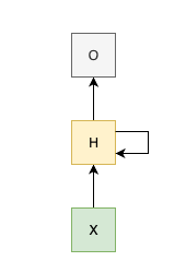
The simplest form of an RNN architecture consists of an input layer, a hidden layer with recurrent connections, and an output layer. The key differentiation from traditional neural networks is that the hidden layer’s output at each time step is fed back into the same hidden layer for the next time step, allowing the network to maintain a form of memory by incorporating information from previous time steps.
See the figure below:
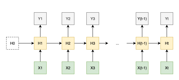
Usually, the architecture can also be represented in an unrolled form, where each time step is shown separately, making it easier to visualize the flow of data input through time.
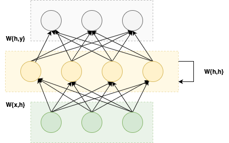
It is also worth to expand the simple form of RNN architecture to show neurons for each layer in its compact form, which can illustrate a direct comparison with traditional feedforward networks.
The mathematical expression for the RNN can be written as follows:
\[\begin{align} h_t &= f(W_{hh} h_{t-1} + W_{xh} x_t + b_h) \\ z_t &= W_{hy} h_t + b_y \tag{1} \\ y_t &= \text{softmax}(z_t) \end{align}\]where:
- \(h_t\) is the hidden state at time \(t\)
- \(x_t\) is the input at time \(t\)
- \(z_t\) is the raw output (logits) at time \(t\)
- \(y_t\) is the output probabilities at time \(t\) after applying softmax
- \(W_{hh}\) is the weight matrix from hidden to hidden (recurrent weights)
- \(W_{xh}\) is the weight matrix from input to hidden
- \(W_{hy}\) is the weight matrix from hidden to output
- \(b_h\) and \(b_y\) are the biases for the hidden and output layers, respectively
- \(f\) is the activation function (commonly tanh or ReLU)
There are a few things to note about the architecture:
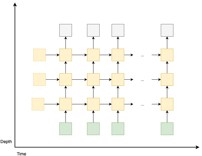
- The architecture demonstrated above is the simplest form with only one hidden layer, so it is not deep at all. However, it can be extended to have multiple hidden layers, similar to deep feedforward networks. And each hidden layer corresponds to a new hidden state, and has its own set of weights and biases.
- For multilayer RNNs, the key structure remains the same: each hidden state at time \(t\) is passed to the next time step \(t+1\) of the same layer \(l\), as well as to the next layer \(l+1\) of current time step \(t\). See the figure below for a simple illustration:
- The weight matrix and biases at each hidden layer are shared across all time steps. This actually is the same as the feedforward neural network, where the weights and biases at each hidden layer are shared across all inputs.
Backpropagation Through Time (BPTT)
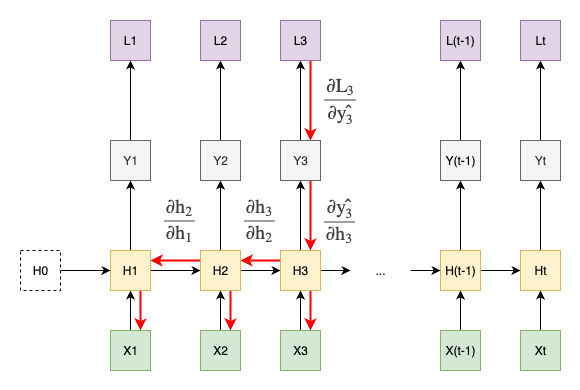
Now, it is the fun part. How backpropagation works in RNNs? Though the concept of backpropagation is similar to that in feedforward networks, the recurrent nature of RNNs introduces a unique characteristic: Backpropagation Through Time (BPTT). This method can be understood by unrolling the RNN through time, treating each time step as a separate layer, and then applying backpropagation as if it were a feedforward network.
See the figure below for a simple illustration which highlights that the gradient of the loss at time step 3 is backpropagated through all previous time steps and then affect the calculation of gradients of weights and biases accordingly.
Let’s define the loss function to be cross-entropy loss at time step \(t\):
\[L_t = -y_{t} \log(\hat{y}_{t}) \tag{2}\]where \(y_{t}\) is the true label and \(\hat{y}_{t}\) is the predicted output at time step \(t\).
Then, the total loss over all time steps is
\[L = \sum_{t} L_t = -\sum_{t} y_{t} \log(\hat{y}_{t}) \tag{3}\]Now, we can compute the gradients of the total loss with respect to the weights and biases in the RNN.
The gradients w.r.t. the weights and biases in output layer can be computed as follows:
\[\begin{align} \frac{\partial L}{\partial W_{hy}} &= \sum_{t} \frac{\partial L_t}{\partial W_{hy}} \\ &= \sum_{t} \frac{\partial L_t}{\partial \hat{y}_{t}} \cdot \frac{\partial \hat{y}_{t}}{\partial z_{t}} \cdot \frac{\partial z_{t}}{\partial W_{hy}} \\ &= \sum_{t} (\hat{y}_{t} - y_{t}) \cdot h_{t}^T \tag{4} \end{align}\] \[\begin{align} \frac{\partial L}{\partial b_y} &= \sum_{t} \frac{\partial L_t}{\partial b_y} \\ &= \sum_{t} \frac{\partial L_t}{\partial \hat{y}_{t}} \cdot \frac{\partial \hat{y}_{t}}{\partial z_{t}} \cdot \frac{\partial z_{t}}{\partial b_y} \\ &= \sum_{t} (\hat{y}_{t} - y_{t}) \tag{5} \end{align}\]📝 Notes
When computing gradients for the softmax cross-entropy loss, it’s much more efficient to calculate the gradient of the loss with respect to the output layer logits \(z_t\) directly. This gives us the clean result \(\frac{\partial L_t}{\partial z_t} = \hat{y}_t - y_t\), rather than computing the gradient with respect to the softmax probabilities \(\hat{y}_t\) and then the gradient from probabilities to logits \(z_t\) as separate steps and multiplying them together.
The calculation of gradients w.r.t. the hidden layer weights and biases is more complex due to the recurrent connections. We need to consider the contributions from all previous time steps that affect the hidden state at time \(t\).
First, we apply the chain rule to expand the gradients calculation as below:
\[\begin{align} \frac{\partial L}{\partial W_{hh}} &= \sum_{t} \frac{\partial L_t}{\partial W_{hh}} \\ &= \sum_{t} \frac{\partial L_t}{\partial \hat{y}_{t}} \cdot \frac{\partial \hat{y}_{t}}{\partial z_{t}} \cdot \frac{\partial z_{t}}{\partial h_{t}} \cdot \frac{\partial h_{t}}{\partial W_{hh}} \tag{6} \end{align}\]Note, $h_t = f(W_{hh} h_{t-1} + W_{xh} x_t + b_h)$, depends on $W_{hh}$ again through the previous hidden state \(h_{t-1}\), which further depends on $W_{hh}$ through hidden state \(h_{t-2}\) and so on. Then, applying chain rule recursively, we can calculate its gradient as follows:
\[\begin{align} \frac{\partial h_t}{\partial W_{hh}} &= \sum_{k=1}^{t} \frac{\partial h_t}{\partial h_k} \cdot \frac{\partial h_k}{\partial W_{hh}} \tag{7} \end{align}\]To obtain equation (7), we need to apply the multivariable chain rule to each time steps inclusive before \(t\). Let’s simplify the notation a bit, and denote \(h_t = f(W_{hh} h_{t-1} + W_{xh} x_t + b_h)\) as \(h_t = f(uv)\), where \(u = W_{hh}\) and \(v = h_{t-1}\). Then, we can apply the multivariable chain rule as follows:
\[\begin{align} \frac{\partial h_t}{\partial W_{hh}} &= \frac{\partial f(uv)}{\partial u} \cdot \frac{\partial u}{\partial W_{hh}} + \frac{\partial f(uv)}{\partial v} \cdot \frac{\partial v}{\partial W_{hh}} \\ &= \frac{\partial f(uv)}{\partial u} \cdot 1 + \frac{\partial f(uv)}{\partial v} \cdot \frac{\partial v}{\partial W_{hh}} \\ &= \frac{\partial f(uv)}{\partial u} + \frac{\partial f(uv)}{\partial h_{t-1}} \cdot \frac{\partial h_{t-1}}{\partial W_{hh}} \text{ ( substituting f(uv) back with h_t )} \\ &= \frac{\partial h_t}{\partial W_{hh}} + \frac{\partial h_t}{\partial h_{t-1}} \cdot \frac{\partial h_{t-1}}{\partial W_{hh}} \tag{8} \end{align}\]\[\begin{align} \frac{\partial h_{t-1}}{\partial W_{hh}} &= \frac{\partial h_{t-1}}{\partial W_{hh}} + \frac{\partial h_{t-1}}{\partial h_{t-2}} \cdot \frac{\partial h_{t-2}}{\partial W_{hh}} \\ \ldots \tag{9} \\ \frac{\partial h_1}{\partial W_{hh}} &= \frac{\partial h_1}{\partial W_{hh}} + 0 \text{ (since h_0 is constant) } \\ &= \frac{\partial h_1}{\partial W_{hh}} \end{align}\]📝 Notes
The left-hand side of equation (8) is the gradient of the hidden state at time step \(t\) with respect to the weights \(W_{hh}\) recursively. The first term on the right-hand side is the direct contribution from the weights at the current time step, while the second term captures how the weights from the previous hidden state \(h_{t-1}\) contributes to the gradient of the current hidden state.
Then, continue calculating partial derivative of \(h_{t-1}\) with respect to \(W_{hh}\) recursively, until we reach the first time step \(h_1\).
Now, we can substitute all equations in (9) back into equation (8) recursively to get the final expression for the gradient of \(h_t\) with respect to \(W_{hh}\):
\[\begin{align} \frac{\partial h_t}{\partial W_{hh}} &= \frac{\partial h_t}{\partial W_{hh}} + \frac{\partial h_t}{\partial h_{t-1}} \cdot \left( \frac{\partial h_{t-1}}{\partial W_{hh}} + \frac{\partial h_{t-1}}{\partial h_{t-2}} \cdot \left( \ldots + \frac{\partial h_1}{\partial W_{hh}} \right) \right) \\ &= \frac{\partial h_t}{\partial W_{hh}} + \frac{\partial h_t}{\partial h_{t-1}} \cdot \frac{\partial h_{t-1}}{\partial W_{hh}} + \frac{\partial h_t}{\partial h_{t-1}} \cdot \frac{\partial h_{t-1}}{\partial h_{t-2}} \cdot \frac{\partial h_{t-2}}{\partial W_{hh}} + \ldots + \frac{\partial h_t}{\partial h_{t-1}} \ldots \frac{\partial h_t}{\partial h_1} \cdot \frac{\partial h_1}{\partial W_{hh}} \tag{10} \\ &= \sum_{k=1}^{t} \left( \prod_{j=k+1}^{t} \frac{\partial h_j}{\partial h_{j-1}} \right) \frac{\partial h_k}{\partial W_{hh}} \end{align}\]where the product term \(\prod_{j=k+1}^{t} \frac{\partial h_j}{\partial h_{j-1}}\) represents the chain of gradients flowing backward from time step \(t\) to time step \(k+1\), and when \(k = t\), this product is defined as 1.
Finally, we can substitute equation (10) back into equation (6) to get the gradient of the loss with respect to \(W_{hh}\):
\[\begin{align} \frac{\partial L}{\partial W_{hh}} &= \sum_{t} \frac{\partial L_t}{\partial W_{hh}} \\ &= \sum_{t} \frac{\partial L_t}{\partial \hat{y}_{t}} \cdot \frac{\partial \hat{y}_{t}}{\partial z_{t}} \cdot \frac{\partial z_{t}}{\partial h_{t}} \cdot \frac{\partial h_{t}}{\partial W_{hh}} \\ &= \sum_{t} (\hat{y}_{t} - y_{t}) \cdot W_{hy}^T \cdot \frac{\partial h_t}{\partial W_{hh}} \\ &= \sum_{t} (\hat{y}_{t} - y_{t}) \cdot W_{hy}^T \cdot \sum_{k=1}^{t} \left( \prod_{j=k+1}^{t} \frac{\partial h_j}{\partial h_{j-1}} \right) \frac{\partial h_k}{\partial W_{hh}} \tag{11} \end{align}\]The gradients with respect to \(W_{xh}\) and \(b_h\) can be calculated in a similar manner. I will ommit the derivation process here, but the final expressions are as follows: \(\begin{align} \frac{\partial L}{\partial W_{xh}} &= \sum_{t} (\hat{y}_{t} - y_{t}) \cdot W_{hy}^T \cdot \sum_{k=1}^{t} \left( \prod_{j=k+1}^{t} \frac{\partial h_j}{\partial h_{j-1}} \right) \frac{\partial h_k}{\partial W_{xh}} \tag{12} \end{align}\)
\[\begin{align} \frac{\partial L}{\partial b_h} &= \sum_{t} (\hat{y}_{t} - y_{t}) \cdot W_{hy}^T \cdot \sum_{k=1}^{t} \left( \prod_{j=k+1}^{t} \frac{\partial h_j}{\partial h_{j-1}} \right) \frac{\partial h_k}{\partial b_h} \tag{13} \end{align}\]Vanishing Gradient Problem
We have already heard about the vanishing gradient problem in the context of training deep neural networks. This issue is particularly pronounced in RNNs due to their recurrent nature.
To understand why, let’s consider the gradients computed in equations (11), (12), and (13). The term \(\prod_{j=k+1}^{t} \frac{\partial h_j}{\partial h_{j-1}}\) represents the product of gradients flowing backward through time.
Let’s calculate this gradient explicitly. Recall that:
\[h_j = f(W_{hh} h_{j-1} + W_{xh} x_j + b_h)\]Taking the derivative with respect to \(h_{j-1}\) and applying the chain rule:
\[\frac{\partial h_j}{\partial h_{j-1}} = f'(W_{hh} h_{j-1} + W_{xh} x_j + b_h) \cdot W_{hh}\]For the common activation functions:
- Tanh: \(f'(z) = 1 - \tanh^2(z)\), which is bounded by \([0, 1]\)
- Sigmoid: \(f'(z) = \sigma(z)(1-\sigma(z))\), which is bounded by \([0, 0.25]\)
- ReLU: \(f'(z) = 1\) if \(z > 0\), else \(0\)
Now, the product becomes:
\[\prod_{j=k+1}^{t} \frac{\partial h_j}{\partial h_{j-1}} = \prod_{j=k+1}^{t} f'(\cdot) \cdot W_{hh}\]Why gradients vanish:
- Activation function derivatives: For tanh and sigmoid, \(f'(\cdot) \leq 1\), often much smaller
- Weight matrix: If the largest eigenvalue of \(W_{hh}\) is less than 1, repeated multiplication will quickly scale down the gradients.
- Long sequences: For a sequence of length \(T\), we multiply up to \(T-1\) terms.
Mathematical analysis: If we assume \(\left|f'(\cdot)\right| \leq \gamma \leq 1\) and \(||W_{hh}|| \leq \lambda\), then:
\[\left|\prod_{j=k+1}^{t} \frac{\partial h_j}{\partial h_{j-1}}\right| \leq (\gamma \lambda)^{t-k}\]So, for \(\gamma \lambda < 1\), this product will decay exponentially as \((t-k)\) increases. Conversely, exploding gradients can occur when \(\gamma \lambda > 1\), causing gradients to grow exponentially, leading to unstable training.
📝 Notes
The vanishing gradient problem doesn’t mean the network can’t learn at all, it just means that it struggles to learn long-term dependencies effectively, which is just illustrated in the analysis above, that the portion of the gradients accumulated from distant time steps through \(\prod_{j=k+1}^{t} \frac{\partial h_j}{\partial h_{j-1}}\) relative to the current time step decays exponentially.
This means that gradients from distant past time steps contribute very little to the weight updates, making it difficult for the RNN to learn long-term dependencies.
There are several techniques to mitigate the vanishing gradient problem so as to learn long-term dependencies, such as Long Short-Term Memory (LSTM) networks and Gated Recurrent Units (GRUs), which introduce gating mechanisms to control the flow of information and gradients. But I won’t cover them in this post, and probably will consider next time.
My Learning Process and Looking Ahead
It is time to self-reflect again on my learning process about new topics like RNNs.
Still, my learning on a specific topic is always driven by curiosity and the desire to understand how things work, as I’ve outlined at the beginning of this post about the questions I want to figure out. I find that having a clear set of questions helps me stay focused and motivated.
My learning structure is usually composed of 2 parts: the grasp of the overall concepts & architecture, and the in-depth understanding of the key components. Returning back to this RNNs topic, following this structure, I first focused on the overall architecture of RNNs and how they differ from traditional feedforward networks. Secondly, I delved into the mathematical details (derivation process) of how backpropagation works in RNNs, as this stays at the core of training RNNs and understanding their limitations, such as the vanishing gradient problem, which motivated the development of more advanced architectures like LSTMs and GRUs, etc.
At the end of this post, looking ahead, though I want to get my hands-on a vanilla RNNs implementations, I can’t wait to start my next learning journey about attention mechanisms, transformers, and modern LLMs. The “Attention is All You Need” paper stays at the top of my reading list, and it very well catches my attention 😊.
References
On this very learning subject, I have referred to the following resources:
Online Courses:
- Stanford Lecture 10 - Recurrent Neural Networks
- MIT 6.S191 (2024): Recurrent Neural Networks, Transformers, and Attention
Blogs:
- The Effectiveness of Recurrent Neural Networks
- Understanding LSTM Networks
- Recurrent Neural Networks Tutorial
Papers:
- Recurrent Neural Networks (RNNs): A gentle Introduction and Overview
- On the difficulty of training Recurrent Neural Networks
- Long Short-Term Memory
Interactive Tools:
- ChatGPT: I used it to clarify my understanding of the concepts and to help me derive the equations for BPTT.